Project WACC and Company WACC

Joachim Kuczynski, 14 November 2025

This article shows how to derive the WACC (weighted average cost of capital) of a project from the WACC of a company (or asset portfolio in general). Further on company and portfolio have the same meaning. Let us assume a company or portfolio with $n$ projects. The relative share of project $i$ in the portfolio is $\alpha_i$ . The WACC of project $i$ is $\omega_i$ . The cost of capital of the portfolio, $\omega_p$ , is given by:

(1) $\begin{equation*}\omega_p=\frac{\sum_{i=1}^{n}V_i\omega_i}{\sum_{j=1}^{n}V_j}=\sum_{i=1}^{n}\frac{V_i}{\sum_{j=1}^{n}V_j}\omega_i=\sum_{i=1}^{n}\alpha_i\omega_i\end{equation*}$

That means that the WACC of a portfolio is the weighted average of the components’ WACC.

Let us have a look at the variance of the portfolio WACC:

(2) $\begin{equation*}\mathrm{var}\left( \omega_p \right)=\mathrm{cov}\left( \omega_p,\omega_p \right)=\mathrm{cov}\left(\sum_{i=1}^{n} \alpha_i\omega_i, \omega_p \right)\end{equation*}$

The covariance is bilinear, we get:

(3) $\begin{equation*}\mathrm{var}\left( \omega_p \right)=\sum_{i=1}^{n}\alpha_i\mathrm{cov}\left( \omega_i, \omega_p \right)\end{equation*}$

The correlation of an asset’s WACC $\omega_i$ with the portfolio’s WACC $\omega_p$ is defined by:

(4) $\begin{equation*}\mathrm{corr}\left( \omega_i,\omega_p \right):=\frac{\mathrm{cov}\left( \omega_i,\omega_p \right)}{\sigma\left( \omega_i \right)\sigma\left( \omega_p \right)}\end{equation*}$

$\sigma (\omega_i)$ and $\sigma (\omega_p)$ are the standard deviations of $\omega_i$ and $\omega_p$ . Substituting covariance by correlation we get:

(5) $\begin{equation*}\mathrm{var}\left( \omega_p \right) =\sum_{i=1}^{n}\alpha_i \sigma \left( \omega_i \right)\sigma\left( \omega_p \right)\mathrm{corr}\left( \omega_i, \omega_p \right)\end{equation*}$

Dividing by the standard deviation $\sigma\left( \omega_p \right)$ leads us to the standard deviation of the portfolio:

(6) $\begin{equation*}\sigma\left( \omega_p \right) =\sum_{i=1}^{n}\alpha_i \sigma \left( \omega_i \right)\mathrm{corr}\left( \omega_i, \omega_p \right)\end{equation*}$

That means that the incremental risk contribution of each project to the risk of the portfolio is $\sigma\left( \omega_i \right)\mathrm{corr}\left( \omega_i, \omega_p \right)$ and not just the weighted sum of its projects’ risks. Hence we can e.g. reduce the WACC of the portfolio by adding a project with negative correlation to the portfolio.\

Instead of including a new project to the portfolio the company can also increase the return of the portfolio by increasing the risk of the portfolio. This reward-to-volatility ratio of the tangential portfolio is given by the Sharpe Ratio:

(7) $\begin{equation*}\frac{\mathbb{E}\left( \omega_p\right)-r_D}{\sigma \left( \omega_p \right)}\end{equation*}$

$\mathbb{E}\left( \omega_p\right)$ is the expected value of $\omega_p$ and $r_D$ is the after-tax debt interest rate. The company wants to invest in the new project, if the additional WACC of this project is lower than an investment in the existing portfolio with the same risk changes. Hence we obtain the requirement to invest in the new project:

(8) $\begin{equation*}\mathbb{E}\left( \omega_i \right)-r_D < \sigma\left( \omega_i \right)\mathrm{corr}\left( \omega_i,\omega_p \right)\frac{\mathbb{E}\left( \omega_p\right)-r_D}{\sigma\left( \omega_p \right)}\end{equation*}$

With that we can define the sensitivity $\beta_i^p$ of the new project to the existing portfolio:

(9) $\begin{equation*}\beta_i^p:=\frac{\sigma\left( \omega_i \right)\mathrm{corr}\left( \omega_i,\omega_p \right)}{\sigma\left( \omega_p \right)}\end{equation*}$

Substituting with $\beta_i^p$ the requirement for the new investment becomes the well-known equation:

(10) $\begin{equation*}\mathbb{E}\left( \omega_i \right) < r_D+\beta_i^p\left( \mathbb{E}\left( \omega_p\right)-r_D \right)\end{equation*}$

With that we can define a maximum annual WACC of the additional project. This is the maximum WACC at which a company would decide to invest in the project.

(11) $\begin{equation*}\mathbb{E}\left( \omega_i \right)^{max} = r_D+\beta_i^p\left( \mathbb{E}\left( \omega_p\right)-r_D \right)\end{equation*}$

Let us assume that the new project and the company are correlated completely, which means $\mathrm{corr}\left( \omega_i,\omega_p \right)=1$ . In this case we get:

(12) $\begin{equation*}\mathbb{E}\left( \omega_i \right)^{max} = r_D+\frac{\sigma\left( \omega_i \right)}{\sigma\left( \omega_p \right)}\left( \mathbb{E}\left( \omega_p\right)-r_D \right)\end{equation*}$

The quotient $\sigma\left( \omega_i \right)/\sigma\left( \omega_p \right)$ is called relative risk factor of project $i$ . The risk premium of the company WACC is adapted by the quotient of the standard deviations of the project and the company. The higher the risk of the project the higher the required WACC of the project to become a new part of the company portfolio. If the risk of the project and the risk of the company are the same, the WACC of the project and the company are the same, too. The standard deviation can be generated by Monte Carlo Simulation or approximated by best/worst case scenarios. Another approach is to estimate the standard deviations by management. Instead of comparing the project to the whole company portfolio we can also compare it to a benchmark project. This benckmark project is considered to be representative for the company.

04/11/202510/11/2025

CAPM Beta and Market Return Rate

Joachim Kuczynski, 04 November 2025

This article is about an unusual sight on the CAPM beta. It provides a derivation from linear regression with the method of least squares. Often the definition of CAPM beta seems to be very abstract. But from the perspective of this article`s approach it might be clearer.

We assume a data set of market return rates $r_{m,i}$ and equity return rates $r_{E,i}$ . $i$ indicates the $i$ -th of $N$ data pairs. $\overline{r_m}$ and $\overline{r_E}$ are the arithmetic mean values of $r_{m,i}$ and $r_{E,i}$ . With the method of least squares we can make a linear regression that approximates the relationship with a linear function $r_E$ .

(1) $\begin{equation*}r_E=a+br_m\end{equation*}$

The slope $b$ of the linear regression function $r_E$ is given by:

(2) $\begin{equation*}b=\frac{\sum_{i=1}^{N}\left( r_{m,i}-\overline{r_m} \right)\left( r_{E,i}-\overline{r_E} \right)}{\sum_{i=1}^{N}\left( r_{m,i}-\overline{r_m} \right)^2}\end{equation*}$

The covariance of $r_m$ and $r_E$ is given by:

(3) $\begin{equation*}\text{cov}(r_E,r_m)=\frac{1}{N-1}\sum_{i=1}^{N}\left( r_{m,i}-\overline{r_m} \right)\left( r_{E,i}-\overline{r_E} \right)\end{equation*}$

The variance of $r_{m}$ is given by:

(4) $\begin{equation*}\text{var}(r_m)=\frac{1}{N-1}\sum_{i=1}^{N}\left( r_{m,i}-\overline{r_m} \right)^2\end{equation*}$

Substituting that in the expression for $b$ leads to:

(5) $\begin{equation*}b=\frac{\text{cov}(r_E,r_m)}{\text{var}(r_m)}\end{equation*}$

This is the same as beta ( $\beta_{r_E}$ ) in the Capital Asset Pricing Model (CAPM). That means that $\beta_{r_E}$ is the slope of the linear approximated relationship of equity return rate $r_E$ and market return rate $r_m$ using the method of least squares. In linear approximation we can state:

(6) $\begin{equation*}b=\beta_{r_E}=\frac{\text{cov}(r_E,r_m)}{\text{var}(r_m)}=\frac{\partial r_E}{\partial r_m}\end{equation*}$

In my point of view this is a very important point to know when doing investment analysis and using CAPM. It provides an additional interpretation of $\beta_{r_E}$ . This point of view is valid for all betas in general.

01/11/202512/11/2025

Operating Leverage

Joachim Kuczynski, 01 November 2025

Net Income

With the abbreviations $\mu$ … net income, S … sales, F … fix expenses, V … variable expenses, A … depreciation and amortization, T … taxes, I … interests for debt and X … tax shield we can define net income by:

(1) $\begin{equation*}\mu=S-F-V-A-T-I+X\end{equation*}$

Let $r_D$ be the interest rate for debt and $r_t$ be the incremental tax rate. We assume that we get full tax shield of $X=Dr_Dr_t$ . Taxes $T$ are paid on EBIT, that means $T=(S-F-V-A ) r_t$ . $Z$ =equity+debt is the asset or enterprise value and d is the debt ratio, $d=D/Z$ . Substituting that in the previous expression we obtain:

(2) $\begin{equation*}\mu=(S-F-V-A)(1-r_t)-dZr_D+dZr_Dr_t\end{equation*}$

Summarizing the terms leads to:

(3) $\begin{equation*}\mu=(S-F-V-A-dZr_D)(1-r_t)\end{equation*}$

Beta of a weighted sum is the weighted sum of the components’ betas, shown in the post “Portfolio Beta”. Thus we get an equation for the betas:

(4) $\begin{equation*}\mu\beta_\mu=(S\beta_S-F\beta_F-V\beta_V-A\beta_A-dZr_D\beta_D)(1-r_t)\end{equation*}$

We assume that fix expenses (F), depreciation, amortization (A) and debt (D) have no correlation to the market return rate, $\beta_F=0$ , $\beta_A=0$ , $\beta_D=0$ . Variable expenses should have the same correlation to market development as sales, that gives $\beta_V=\beta_S$ . We obtain:

(5) $\begin{equation*}\mu \beta_\mu=\left( S-V \right) \left( 1-r_t \right) \beta_S\end{equation*}$

Substituting $\mu=\left( S-F-V-A -dZr_D \right) \left( 1-r_t \right)$ leads to:

(6) $\begin{equation*}\beta_\mu= \frac{ S-V }{ S-F-V-A -dZr_D }\beta_S\end{equation*}$

Rearranging the terms shows:

(7) $\begin{equation*}\beta_\mu=\left( 1+ \frac{ F+A+dZr_D }{ S-F-V-A -dZr_D } \right) \beta_S\end{equation*}$

Return on Equity

Return on equity measures relative equity increase. It is defined by:

(8) $\begin{equation*}\text{ROE}=\frac{\text{net income}}{\text{equity}}=\frac{\mu}{(1-d)Z}\end{equation*}$

With the substitution of $\mu$ we obtain:

(9) $\begin{equation*}\text{ROE}=\frac{\left( S-F-V-A-dZr_D \right)(1-r_t) }{(1-d)Z}\end{equation*}$

We want to link the beta of ROE to the beta of net income. We take the definition of $\beta$ with its bilinearity of covariance and get:

(10) $\begin{equation*}\beta_{\text{ROE}}=\frac{cov(r_\frac{\mu}{E}, r_m)}{var(r_m)}=\frac{\frac{1}{E}cov(r_\mu, r_m)}{var(r_m)}=\frac{1}{E}\beta_\mu=\frac{1}{(1-d)Z}\beta_\mu\end{equation*}$

Hence we get $\beta_{\text{ROE}}$ as function of $\beta_S$ :

(11) $\begin{equation*}\beta_{\text{ROE}}=\left(\frac{ S-V }{ S-F-V-A -dZr_D}\right)\frac{1}{(1-d)Z}\beta_S\end{equation*}$

(12) $\begin{equation*}\beta_{\text{ROE}}=\left( 1+ \frac{ F+A+dZr_D }{ S-F-V-A -dZr_D}\right)\frac{1}{(1-d)Z}\beta_S\end{equation*}$

This is the relationship of the ROE beta and the sales beta. It depends on several variables, but especially on fixed expenses $F+A+dZr_D$ .

Releveraging Equity Return Rate and WACC

An equity investor wants to know which return rate market provides at the same risk (volatility) level as our investigated investment. The WACC after taxes of the appropriate market portfolio is given by:

(13) $\begin{equation*}\text{WACC'}=d'r_D'\left( 1-r_t' \right)+(1-d')r_{E'}\end{equation*}$

I indicate all market portfolio parameters with a line on the top. $r_{E'}$ ist the required return rate of an incremental equity investor. This is the return rate of the completely diversified market portfolio of the appropriate industry segment. The Capital Asset Pricing Model (CAPM) states that $r_{E'}$ can be approximated by a linear function of $\beta_{E'}$ by a given market return rate $r_m$ :

(14) $\begin{equation*}r_{E'}=r_f+\beta_{E'}\left( r_m-r_f \right); \beta_{E'}=\frac{cov(r_{E'},r_m)}{var(r_m)}\end{equation*}$

$\beta_{E'}$ is the average equity $\beta$ of an market portfolio representing the investigated investment. It is based on an averaged financial and operating leverage of the market portfolio. If these parameters do not match capital and cost structure of the considered investment, you have to “releverage” $\beta_{E'}$ .

Operating leverage: We have a look at the relationship of $\beta_{E'}$ and $\beta_{S'}$ :

(15) $\begin{equation*}\beta_{\text{E'}}=\left(\frac{ S-V' }{ S'-F'-V'-A' -d'Z'r_D'}\right)\frac{1}{(1-d')Z'}\beta_{S'}\end{equation*}$

$\beta_{E'}$ is provided by an official data collection in most cases. With the other data from the market portfolio we can calculate $\beta_{S'}$ :

(16) $\begin{equation*}\beta_{\text{S'}}=\left(\frac{ S'-F'-V'-A' -d'Z'r_{D'} }{S'-V'}\right)(1-d')Z'\beta_{E'}\end{equation*}$

$\beta_{S'}$ is the linear approximated change of sales because of a change in market return rate $r_m$ . $\beta_{S'}$ does not depend on $F$ , $V$ , $Z$ , $D$ , $d$ and $r_D$ . $\beta_{S'}$ is the same for all combinations of these parameters, that means $\beta_S=\beta_{S'}$ . Now we take the parameters of the investment, to which we want to adjusted $\beta_E$ . With the $\beta_{S'}$ from the previous equation we obtain the adjusted $\beta_E$ :

(17) $\begin{equation*}\beta_{\text{E}}=\left(\frac{ S-V }{ S-F-V-A-dZr_D}\right)\frac{1}{(1-d)Z}\beta_S\end{equation*}$

With this $\beta_E$ we can calculate the new equity return rate $r_E$ :

(18) $\begin{equation*}r_E=r_f+\beta_E\left( r_m-r_f \right)\end{equation*}$

After the releveraging process we get the releveraged WACC with the appropriate $r_E$ :

(19) $\begin{equation*}\text{WACC}=dr_D\left( 1-r_t \right)+(1-d)r_E\end{equation*}$

05/10/202501/11/2025

Financial Lease Valuation

Joachim Kuczynski, 05 October 2025

Standard Evaluation

In this post I would like to explain how to evaluate a financial lease contract. Most lease contracts in economic life are financial lease ones. Financial lease payments are fixed obligations equivalent to debt service. Financial lease is just another way of borrowing money to pay for an asset. I provide an example to explain the standard evaluation procedure.

We want to decide whether it is better to make an investment $I$ of 100 thousand Euro (k€) or to lease it with annual payments of 12.5 k€. The investment is usable for 10 years and has a no salvage value. The lease payments have to be done in advance and are constant over 10 years. In the table below you can see the consequences of leasing the asset compared to make the investment. Leasing reduces your depreciation, and as a consequence the tax shield because of depreciation is lost. On the other hand the lease payments are fully tax-deductible. We discount the cash flows by the company’s borrowing rate. We can deduct the interest payments from the taxable income. Hence the net cost of borrowing is the after-tax interest rate. So the after-tax interest rate is the effective rate at which a company can transfer debt-equivalent cash flows from one time period to another. With an interest rate $r_d$ , a tax rate $r_t$ and (to investment) differing leasing cash flows $C_t$ we get the net value of lease $V_l$ :

$V_l=I-\sum_{t=0}^{n}\frac{C_t}{\left( 1+r_d \left(1-r_t \right)\right)^t}$

$V_l>0$ means that leasing is better than doing the investment, $V_l<0$ indicates that leasing is worse than investing.

In an additional table you can see the calculation of the equivalent loan leading to the same cash flows as the leasing contract. In our example $V_l$ is 3.8 k€. That means that leasing is better than investing and should be preferred.

$I$ can be a single investment value, but also the NPV of an investment cash flow sequence, discounted by the debt interest rate. You can also take yearly investment cash flows .

In general you should take care whether the company can really receive full tax shield and whether payments in a yearly time scale is sufficiently precise. If you have additional cash flows for maintenance, insurance, salvage value, etc., you can simply add it to the cash flows. The procedure remains the same.

Maintenance and salvage value are harder to predict than the other cash flows. If the risk, or volatility respectively, is significantly higher it might be better to discount them with a higher, risk-adjusted discount rate. CAPM helps to provide appropriate discount rates.

Separation and Project Implementation

Next we want to seperate the investment and leasing scenario. This must lead to the same result, because the present values are additive and separable. In the following table the investment and leasing scenarios are evaluated by their own. The result ist the same, NPV of financial leasing is 8.3 k€ better than investing.

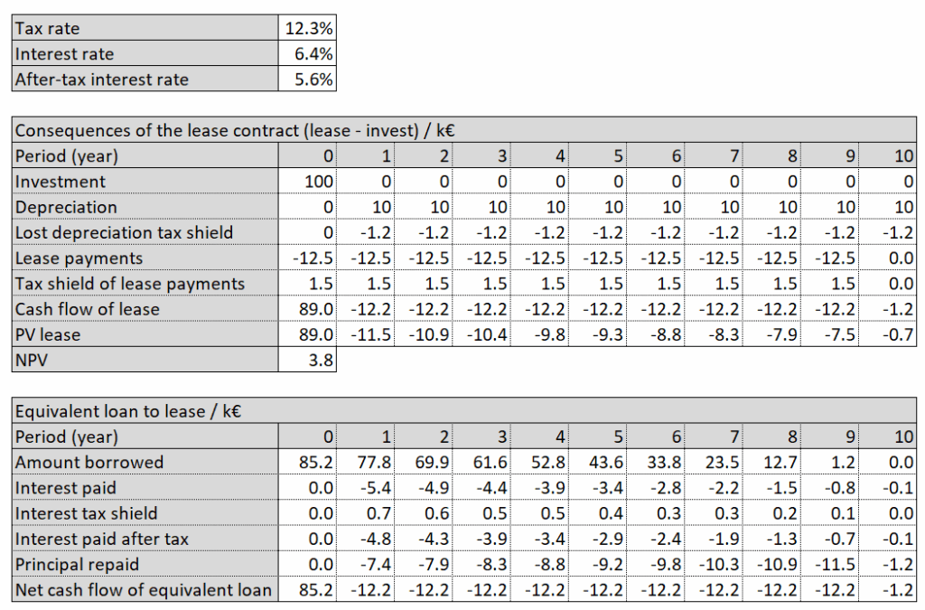
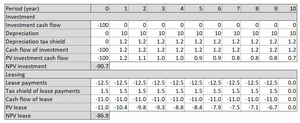
Let $C_{i,t}$ be the investment scenario cash flow and $C_{l,t}$ be the lease cash flow in period t. If we discount all cash flows with the same discount rate, the interest rate after taxes in our case, we can separate:

$\sum_{t=0}^{n}\frac{\left( C_{i,t} - C_{l,t} \right)}{\left( 1+r_d \left(1-r_t \right)\right)^t}=$

$=\sum_{t=0}^{n}\frac{ C_{i,t}}{\left( 1+r_d \left(1-r_t \right)\right)^t}-\sum_{t=0}^{n}\frac{C_{l,t}}{\left( 1+r_d \left(1-r_t \right)\right)^t}$

I prefer this separate analysis. This allows to take different discount rates for the cash flows with higher volatilities, or risks respectively, e.g. maintenance and salvage value. If you discount just the cash flow differences, you cannot do that easily. And you can proceed further analysis much easier with separate analysis data.

After you have decided whether you want do buy or lease, you probably intend do implement this decision in an overall project valuation. Then you have to transfer the corresponding cash flows in that valuation and discount with the same discount rates. This procedure can easily lead to failures if you do not use NPV with the component cash flow procedure as decision figure. If you discount the project with only one “company WACC” (project cash flow procedure) for example, this will provide false results. Additionally you can get implementation problems using project return rates as decision figure. But that is another story.

27/11/202427/11/2024

Discount Rate vs. Capitalization Rate

Joachim Kuczynski, 27 November 2024

The valuation of investments and projects (or assets in general) is based on shifting and adjusting cash flows on the time axis. A shift backwards in time is called discounting. A shift forwards in time is called capitalization. Many analysts use the same rate for discounting and capitalization when valuing a project. But can you really shift the cash flows back and forth on the time axis at the same rate? The answer to this is a clear no.

The discount rate of a cash flow is based on its inherent risk (volatility). In general, it does not depend on the risk preferences of the capital providers, when their investment portfolio is diversified sufficiently. The capitalization rate of a cash flow, on the other hand, is based on the risk preferences and portfolio diversification of the company (or its capital providers). The capitalization rate does not depent on the inherent risk of the initial cash flow. Once it is available for capitalization, it does not matter under what circumstances it came about. Discount rates and capitalization rates are fundamentally different. Taking the same rate in calculations is a fundamental, logical error.

There are key figures for investment valuation that include a recapitalization of returning cash flows. A well-known example is the modified internal rate of return or the Baldwin rate. It is usually assumed that both discounting and reinvestment are carried out using the same rate, the WACC. The WACC is based on the return expectations of the capital providers. However, these do not necessarily have to correspond to the return opportunities of the investing company. Additional rates (“risk premiums”) are often added to the discount rate. This is intended to take currency or location risks into account, for example. If you now use the same rate for capitalization, you assume an increased reinvestment rate for the company. This makes no sense and increases the error in the investment calculation.

In summary, we can state that equating discount rate and capitalization rate is fundamentally wrong. Many formulas are simplified by equating these two rates. But it is simply wrong, anyway. The results of the calculation are no longer valid doing that. However, correct and meaningful results of the investment calculation are the basis for correct investment decisions. So take care and do not simplify what cannot be simplified. Economic reality is complex, and their calculations can be too.