Joachim Kuczynski, 01 November 2025
Net Income
With the abbreviations  … net income, S … sales, F … fix expenses, V … variable expenses, A … depreciation and amortization, T … taxes, I … interests for debt and X … tax shield we can define net income by:
(1) 
Let  be the interest rate for debt and
  be the incremental tax rate. We assume that we get full tax shield of
  . Taxes
  are paid on EBIT, that means
  .
.  =equity+debt is the asset or enterprise value and d is the debt ratio,
  . Substituting that in the previous expression we obtain:
(2) 
Summarizing the terms leads to:
(3) 
Beta of a weighted sum is the weighted sum of the components’ betas, shown in the post “Portfolio Beta”. Thus we get an equation for the betas:
(4) 
We assume that fix expenses (F), depreciation, amortization (A) and debt (D) have no correlation to the market return rate,  ,
,  ,
,  . Variable expenses should have the same correlation to market development as sales, that gives
  . We obtain:
(5) 
Substituting  leads to:
(6) 
Rearranging the terms shows:
(7) 
Return on Equity
Return on equity measures relative equity increase. It is defined by:
(8) 
With the substitution of we obtain:
(9) 
We want to link the beta of ROE to the beta of net income. We take the definition of  with its bilinearity of covariance and get:
(10) 
Hence we get  as function of
  :
:
(11) 
(12) 
This is the relationship of the ROE beta and the sales beta. It depends on several variables, but especially on fixed expenses  .
.
Releveraging Equity Return Rate and WACC
An equity investor wants to know which return rate market provides at the same risk (volatility) level as our investigated investment. The WACC after taxes of the appropriate market portfolio is given by:
(13) 
I indicate all market portfolio parameters with a line on the top.  ist the required return rate of an incremental equity investor. This is the return rate of the completely diversified market portfolio of the appropriate industry segment. The Capital Asset Pricing Model (CAPM) states that can be approximated by a linear function of
  by a given market return rate
  :
:
(14) 
is the average equity of an market portfolio representing the investigated investment. It is based on an averaged financial and operating leverage of the market portfolio. If these parameters do not match capital and cost structure of the considered investment, you have to “releverage” .
Operating leverage: We have a look at the relationship of and  :
:
(15) 
is provided by an official data collection in most cases. With the other data from the market portfolio we can calculate :
(16) 
is the linear approximated change of sales because of a change in market return rate . does not depend on  ,
,  , ,
, ,  ,
,  and . is the same for all combinations of these parameters, that means
  . Now we take the parameters of the investment, to which we want to adjusted
  . With the from the previous equation we obtain the adjusted :
(17) 
With this we can calculate the new equity return rate  :
:
(18) 
After the releveraging process we get the releveraged WACC with the appropriate :
(19) 
 . With that we obtain
  .
. is:
is:![\[ r_v=r_f+\beta_v\left( r_m-r_f \right) \]](https://www.financeinvest.at/wp-content/ql-cache/quicklatex.com-3ee7dd71a1607b3846dc46be0f328058_l3.png "Rendered by QuickLaTeX.com")
![\[ r_a=r_f+\beta_a\left( r_m-r_f \right) \]](https://www.financeinvest.at/wp-content/ql-cache/quicklatex.com-da3fa7396c5319603d30e5fe815e0726_l3.png "Rendered by QuickLaTeX.com")
![\[ r_v=r_a-r_f-\beta_a\left( r_m-r_f \right) + r_f+ \beta_v \left( r_m-r_f \right) \]](https://www.financeinvest.at/wp-content/ql-cache/quicklatex.com-63a0adfe7e092809b959ab3e12ab1ad8_l3.png "Rendered by QuickLaTeX.com")
![\[ r_v=r_a- \left( r_m-r_f \right) \left( \beta_a -\beta_v \right) \]](https://www.financeinvest.at/wp-content/ql-cache/quicklatex.com-7efc5a713f9f9b0200bdddf5a9b9fcb7_l3.png "Rendered by QuickLaTeX.com")
![\[ \beta_a=\beta_f\frac{-\left| V_f \right|}{V_a}+\beta_v\frac{V_v}{V_a}=\beta_v\frac{V_v}{V_a} \]](https://www.financeinvest.at/wp-content/ql-cache/quicklatex.com-e5bf1006a9a0fce83b6285ba495466dd_l3.png "Rendered by QuickLaTeX.com")
![\[ \beta_a - \beta_v = \beta_a \left( 1-\frac{V_a}{V_v} \right) =\beta_a \frac{ \left| V_f \right| }{ \left| V_f \right| + V_a} \]](https://www.financeinvest.at/wp-content/ql-cache/quicklatex.com-8b5c6ac60c6d868aabba62975ed83ee1_l3.png "Rendered by QuickLaTeX.com")
![\[ r_v=r_a- \left( r_m-r_f \right) \beta_a \frac{ \left| V_f \right| }{ \left| V_f \right| + V_a} \]](https://www.financeinvest.at/wp-content/ql-cache/quicklatex.com-54e8e369fbe58654da69b8d7e1862eb5_l3.png "Rendered by QuickLaTeX.com")
 by
by  leads to the final result:
![\[ r_v= r_a- \left( r_a-r_f \right) \frac{ \left| V_f \right| }{ \left| V_f \right| + V_a}\]](https://www.financeinvest.at/wp-content/ql-cache/quicklatex.com-9f2ca73ccd5fd37c03e2e0248bc329a7_l3.png "Rendered by QuickLaTeX.com")
 in the previous formula gives:
![\[ r_v\left( V_f = 0 \right) = r_a \]](https://www.financeinvest.at/wp-content/ql-cache/quicklatex.com-e4f47b2c6bc8971d7a56ce97413b5de6_l3.png "Rendered by QuickLaTeX.com")
![\[ r_v\left( V_a = 0 \right) = r_f \]](https://www.financeinvest.at/wp-content/ql-cache/quicklatex.com-2bb9db0ca6cadc95506696b31c1e081b_l3.png "Rendered by QuickLaTeX.com")
 of 100 thousand Euro (k€) or to lease it with annual payments of 12.5 k€. The investment is usable for 10 years and has a no salvage value. The lease payments have to be done in advance and are constant over 10 years. In the table below you can see the consequences of leasing the asset compared to make the investment. Leasing reduces your depreciation, and as a consequence the tax shield because of depreciation is lost. On the other hand the lease payments are fully tax-deductible. We discount the cash flows by the company’s borrowing rate. We can deduct the interest payments from the taxable income. Hence the net cost of borrowing is the after-tax interest rate. So the after-tax interest rate is the effective rate at which a company can transfer debt-equivalent cash flows from one time period to another. With an interest rate
  , a tax rate
  we get the net value of lease
  :
:![\[V_l=I-\sum_{t=0}^{n}\frac{C_t}{\left( 1+r_d \left(1-r_t \right)\right)^t}\]](https://www.financeinvest.at/wp-content/ql-cache/quicklatex.com-2a7aa6733405981af5a4daba9e405359_l3.png "Rendered by QuickLaTeX.com")
 means that leasing is better than doing the investment,
  indicates that leasing is worse than investing.
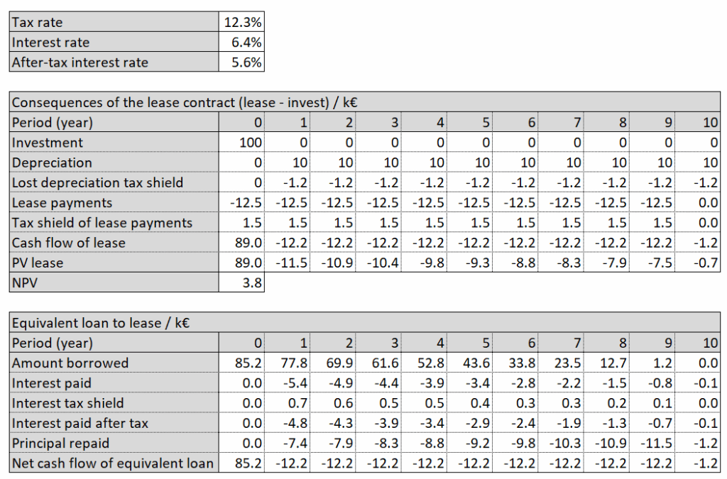
 be the investment scenario cash flow and
  be the lease cash flow in period t. If we discount all cash flows with the same discount rate, the interest rate after taxes in our case, we can separate:
![\[\sum_{t=0}^{n}\frac{\left( C_{i,t} - C_{l,t} \right)}{\left( 1+r_d \left(1-r_t \right)\right)^t}=\]](https://www.financeinvest.at/wp-content/ql-cache/quicklatex.com-bbdbe0b0f75b2a0f8bed462292847df8_l3.png "Rendered by QuickLaTeX.com")
![\[=\sum_{t=0}^{n}\frac{ C_{i,t}}{\left( 1+r_d \left(1-r_t \right)\right)^t}-\sum_{t=0}^{n}\frac{C_{l,t}}{\left( 1+r_d \left(1-r_t \right)\right)^t}\]](https://www.financeinvest.at/wp-content/ql-cache/quicklatex.com-c1d6f85415bf645b3bede9acb1b6f5c1_l3.png "Rendered by QuickLaTeX.com")
 is defined by:
![\[\beta_p=\frac{cov(r_p,r_m)}{var(r_m)}\]](https://www.financeinvest.at/wp-content/ql-cache/quicklatex.com-d4ef4da8f1e8ab77a034e0b8da002c38_l3.png "Rendered by QuickLaTeX.com")
 , is the weighted average of its components’ return rates:
![\[r_p=\sum_{i=1}^{n}\alpha_ir_i\]](https://www.financeinvest.at/wp-content/ql-cache/quicklatex.com-7a58dd9b270e96a227c4ced12ba0b223_l3.png "Rendered by QuickLaTeX.com")
 stands for the relative value share of asset
  in the portfolio. The covariance of two random variables is bilinear. Hence we get:
![\[cov(r_p, r_m)=cov(\sum_{i=1}^{n}\alpha_ir_i,r_m)=\sum_{i=1}^{n}\alpha_icov(r_p, r_m)\]](https://www.financeinvest.at/wp-content/ql-cache/quicklatex.com-10de1be8e0635eb826fdc60bf0e5ed6b_l3.png "Rendered by QuickLaTeX.com")
![\[\beta_p=\frac{\sum_{i=1}^{n}\alpha_icov(r_p, r_m)}{var(r_m)}=\sum_{i=1}^{n}\alpha_i\beta_i\]](https://www.financeinvest.at/wp-content/ql-cache/quicklatex.com-6678a30fba9b392c30156bc1a214cd77_l3.png "Rendered by QuickLaTeX.com")
 assets is the weighted average of its components, weighted by their relative value share in the portfolio.
 .
. .
. and the yearly fixed cash flow is
  . Both cash flows are estimated to occur at the end of each year, beginning in year 1. The yearly cash flow of the asset is
  . Assuming infinite periods we get a perpetuity and can apply the formula of convergent geometric series.
 is the present value of
  discounted with
  is the present value of
  is the present value of
  is the present value of
  is the present value of
 ![\[ V_a^a = \frac{C_a}{r_a}, V_f^a=\frac{C_f}{r_a}, V_f^f=\frac{C_f}{r_f},V_v^a=\frac{C_v}{r_a},V_v^v=\frac{C_v}{r_v} \]](https://www.financeinvest.at/wp-content/ql-cache/quicklatex.com-a5e1ac4bc9c18e87411a96b62844a496_l3.png "Rendered by QuickLaTeX.com")
 has to be the same when we discount all cash flows with the asset discount rate
 ![\[ V_a^a=V_v^a+V_f^a=V_f^f+V_v^v \]](https://www.financeinvest.at/wp-content/ql-cache/quicklatex.com-3206dc15e5c646023b4aa2e93680a8e8_l3.png "Rendered by QuickLaTeX.com")
![\[ r_v=\frac{r_a}{1-\frac{C_f}{C_v}\left( \frac{r_a}{r_f}-1 \right)} \]](https://www.financeinvest.at/wp-content/ql-cache/quicklatex.com-95872d0a31aa511d42eef9c28dd1a8bb_l3.png "Rendered by QuickLaTeX.com")
 and not on their absolute values.
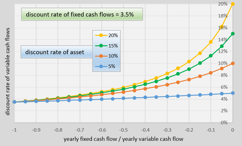
 the
the  Obviously that is true, because asset and variable cash flows and hence also their discount rates are the same.
 from databases in literature or in the web. In my articles concerning
 ![\[\beta^{ind}_{rev}=\beta ^{ind}_{asset} \left( 1-\frac{V^{ind}_{fix}}{V^{ind}_{asset}} \right)^{-1}\]](https://www.financeinvest.at/wp-content/ql-cache/quicklatex.com-cde5ba671ecc1b7b10012fd92a965c0e_l3.png "Rendered by QuickLaTeX.com")
 . Hence we obtain:
![\[\beta^{proj}_{rev}=\beta ^{ind}_{asset} \left( 1-\frac{V^{ind}_{fix}}{V^{ind}_{asset}} \right)^{-1}\]](https://www.financeinvest.at/wp-content/ql-cache/quicklatex.com-353eccdb29a981373f6cdc4bca2ce048_l3.png "Rendered by QuickLaTeX.com")
![\[\beta^{proj}_{asset}=\beta ^{proj}_{rev} \left( 1-\frac{V^{proj}_{fix}}{V^{proj}_{asset}} \right)=\]](https://www.financeinvest.at/wp-content/ql-cache/quicklatex.com-f653639fde45c24bb671287829805624_l3.png "Rendered by QuickLaTeX.com")
![\[= \beta ^{ind}_{asset} \frac{1-\frac{V^{proj}_{fix}}{V^{proj}_{asset}}}{1-\frac{V^{ind}_{fix}}{V^{ind}_{asset}}}\]](https://www.financeinvest.at/wp-content/ql-cache/quicklatex.com-2e59a7922907e0e1cf633939c849f6b1_l3.png "Rendered by QuickLaTeX.com")
![\[\beta^{project}_{asset}=1.0 \left( 1+ \frac {1000}{200} \right)=6\]](https://www.financeinvest.at/wp-content/ql-cache/quicklatex.com-e757d8c2543eaf64339e1fdf4bef1aed_l3.png "Rendered by QuickLaTeX.com")
![\[\beta_{P}=\frac{R}{R-C}\beta_{R} - \frac{C}{R-C}\beta_{C}=\]](https://www.financeinvest.at/wp-content/ql-cache/quicklatex.com-214f6b4aa833f50c0348169b35112362_l3.png "Rendered by QuickLaTeX.com")
![\[=\frac{1200}{1200-1000}1 - \frac{1000}{1200-1000}0=6\]](https://www.financeinvest.at/wp-content/ql-cache/quicklatex.com-58210695bcd89b8fbc6f9c8b560ad8fa_l3.png "Rendered by QuickLaTeX.com")
 , variable costs
  and revenues
  cannot be found easily. But we can try to approximate them with P&L or balance sheet figures, which are available more eaysily. Let us consider eternal yearly revenues
  , yearly fixed costs
  and yearly variable costs
  . The risk free rate is
 ![\[\beta _{asset} = \beta_{rev} \left( 1 - \frac{V_{fix}}{V_{asset}} \right) \]](https://www.financeinvest.at/wp-content/ql-cache/quicklatex.com-1dfd5750e036dfe0ed0c2580165d58d1_l3.png "Rendered by QuickLaTeX.com")
![\[V_{fix}=- \frac{\alpha R}{r_f}\]](https://www.financeinvest.at/wp-content/ql-cache/quicklatex.com-8c2173bb867d2039c7c24b01280886db_l3.png "Rendered by QuickLaTeX.com")
![\[V_{asset}= \frac{R - \alpha R - \beta R}{r_m}\]](https://www.financeinvest.at/wp-content/ql-cache/quicklatex.com-2047a4c2ba3b0169ee09b36933d3035a_l3.png "Rendered by QuickLaTeX.com")
 :
:![\[\beta _{asset} = \beta_{rev} \left( 1 + \frac{\frac{\alpha R}{r_f}}{\frac{R - \alpha R - \beta R}{r_m}} \right) = \beta_{rev} \left( 1 + \frac{r_m}{r_f}\frac{\alpha}{1-\alpha-\beta} \right) \]](https://www.financeinvest.at/wp-content/ql-cache/quicklatex.com-2d2c815f15ff7b3feca76b5a7bb8316c_l3.png "Rendered by QuickLaTeX.com")
 and
and  approximately, so
  ,
,  is the ratio of annual fixed costs to annual profit. That means that you have to multiply that factor with the 2, when applying P&L figures in approximation and not present values.
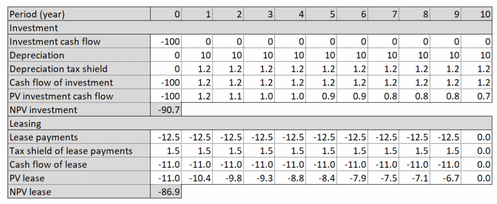
  for the buying and
  for the leasing scenario). Adding up all present values you get a net present value (NPV) of the buying case and a NPV of the leasing case.
![\[NPV_b=\sum_{i}^{}\gamma_{b,i}C_{b,i}\]](https://www.financeinvest.at/wp-content/ql-cache/quicklatex.com-7edf54aa8061c21fae0649b7cb42febf_l3.png "Rendered by QuickLaTeX.com")
![\[NPV_l=\sum_{j}^{}\gamma_{l,j}C_{l,j}\]](https://www.financeinvest.at/wp-content/ql-cache/quicklatex.com-2ff141704520007119cf9e00400279cc_l3.png "Rendered by QuickLaTeX.com")
 .
. ,
,  , which is the sum of different assets values
  :
:![\[C(t)=\sum_{i}^{}C_i(t)\]](https://www.financeinvest.at/wp-content/ql-cache/quicklatex.com-238c5682b36c90200f3872ee0001a260_l3.png "Rendered by QuickLaTeX.com")
 the asset values are
  and
and  with
with  . The asset value
  is developing in time
  , that means:
![\[C_i (t)=C_i(0)exp(r_i t)\]](https://www.financeinvest.at/wp-content/ql-cache/quicklatex.com-199dec8af5bafc55f69c19ffd13b2d2b_l3.png "Rendered by QuickLaTeX.com")
 , that describes the development of the aggregated asset value
  . Setting
  we obtain:
![\[r=\frac{1}{t}ln\frac{C(t)}{C(0)}=\frac{1}{t}ln\left( \sum_{i}^{} \left \frac{C_i(0)}{C(0)} exp \left( r_i t \right) \right \right)\]](https://www.financeinvest.at/wp-content/ql-cache/quicklatex.com-fb659cb84b82fa3fac2f0009b503dd4b_l3.png "Rendered by QuickLaTeX.com")
 and
and  . Hence we get a first order approximation of
 ![\[r\simeq \frac{1}{t}\left( \sum_{i}^{} \left( \frac{C_i(0)}{C(0)} \left( 1+ r_i t \right) \right) -1 \right)\]](https://www.financeinvest.at/wp-content/ql-cache/quicklatex.com-87db3d07482630425a989b6495027b30_l3.png "Rendered by QuickLaTeX.com")
![\[r\simeq \sum_{i}^{} \frac{C_i(0)}{C(0)} r_i\]](https://www.financeinvest.at/wp-content/ql-cache/quicklatex.com-5806f016a86a9e819753e1a5e6579448_l3.png "Rendered by QuickLaTeX.com")
 return rate
 ![\[WACC=r=\frac{D}{E+D}r_D+\frac{E}{E+D}r_E\]](https://www.financeinvest.at/wp-content/ql-cache/quicklatex.com-7b9fcbf01c1f74e6a122461f37027337_l3.png "Rendered by QuickLaTeX.com")
 or
or  . With a substitution of
  , you can transform these two return rates into each other.
 , is the sum of revenues’ value,
 ![\[V_{asset}=V_{rev}+V_{var}+V_{fix}\]](https://www.financeinvest.at/wp-content/ql-cache/quicklatex.com-cf23103bfba3ed586bd4ee1464a7b4d8_l3.png "Rendered by QuickLaTeX.com")
![\[\beta_{asset}=\frac{\beta_{rev} V_{rev} + \beta_{var} V_{var}+ \beta_{fix} V_{fix}}{V_{asset}}.\]](https://www.financeinvest.at/wp-content/ql-cache/quicklatex.com-f9abbfbe3a34248c1ea171096730d969_l3.png "Rendered by QuickLaTeX.com")
 and therefore
  . We obtain:
![\[\beta_{asset}=\frac{V_{rev}\beta_{rev} + V_{var}\beta_{var}}{V_{asset}}\]](https://www.financeinvest.at/wp-content/ql-cache/quicklatex.com-c8bd7662c544e7ee1cc1dfd493bc7da0_l3.png "Rendered by QuickLaTeX.com")
 . We get:
![\[\beta_{asset}=\beta_{rev} \frac{V_{rev} + V_{var}}{V_{asset}}=\beta_{rev} \left( 1-\frac{V_{fix}}{V_{asset}} \right)\]](https://www.financeinvest.at/wp-content/ql-cache/quicklatex.com-460385135a1bed426f4e8cc7f7cb9662_l3.png "Rendered by QuickLaTeX.com")
 , and the value of the asset is positive,
  , in ordinary cases. The expression in the bracket becomes
  . That means that the beta of the asset is higher than the beta of the revenues,
  . Obviously that is true, because adding fixed costs increases the beta of the asset. This effect is known as operating leverage.
 and
and  .
. ![\[r_E=r_f+\beta _{rev}\left( r_m - r_f \right)\]](https://www.financeinvest.at/wp-content/ql-cache/quicklatex.com-333b7bf948d2e673718fe660bee9b387_l3.png "Rendered by QuickLaTeX.com")
 considering debt
 ![\[r_{rev}=\frac{D}{E+D} \left( 1-t \right) r_D + \frac{E}{E+D} r_E\]](https://www.financeinvest.at/wp-content/ql-cache/quicklatex.com-8816ce85e3ebb914b2b3b891bb1d463d_l3.png "Rendered by QuickLaTeX.com")
 , divided by the present value of all investment cash flows,
  . Hereby it is important how we define the term investment. You can have a look at my proposal in this
 ![\[PI=\frac{PV_C}{PV_I}\]](https://www.financeinvest.at/wp-content/ql-cache/quicklatex.com-f8912a2a1acef3578476fece21ce73f7_l3.png "Rendered by QuickLaTeX.com")
 shows how much value is created per investment. All projects with a
  are creating additional value to the investors, all projects with a
  are destroying value.
![\[PI^*=\frac{PV_C-PV_I}{PV_I}=\frac{PV_C}{PV_I}-1=PI-1\]](https://www.financeinvest.at/wp-content/ql-cache/quicklatex.com-852d8bdcfe0d8e08d8e4e08ea95efc33_l3.png "Rendered by QuickLaTeX.com")
 :
:![\[PIA=\frac{PI}{A_{n,r}}\]](https://www.financeinvest.at/wp-content/ql-cache/quicklatex.com-cae3fb545351871cad5018e3c01b814b_l3.png "Rendered by QuickLaTeX.com")
![\[A_{n,r}=\frac{1}{r}\left( 1-\frac{1}{\left( 1+r \right)^n} \right)\]](https://www.financeinvest.at/wp-content/ql-cache/quicklatex.com-bb804176bdcf6a6e5abb0a6b97de6a61_l3.png "Rendered by QuickLaTeX.com")
![\[I_t^{res}:=f_t+c_t-c_{t-1}-c_{t-1}i_t\]](https://www.financeinvest.at/wp-content/ql-cache/quicklatex.com-bc65d4df301a3c2e176603cf8e26139f_l3.png "Rendered by QuickLaTeX.com")
 is the cash flow in period
  the fixed capital in period
  the discount rate in period
  is just the depreciation in period
 ![\[\sum_{t=0}^{n}(f_t-I_t^{res})\rho_t=\sum_{t=0}^{n}(c_{t-1}(1+i_t)-c_t)\rho_t\]](https://www.financeinvest.at/wp-content/ql-cache/quicklatex.com-69a2df2c6eec9bcf4204b280e7e4d618_l3.png "Rendered by QuickLaTeX.com")
 is the discount factor in period
  . That means
  . With that we obtain:
![\[\sum_{t=0}^{n}(f_t-I_t^{res})\rho_t=\sum_{t=0}^{n}(c_{t-1}\rho_{t-1} - c_t \rho_t)\]](https://www.financeinvest.at/wp-content/ql-cache/quicklatex.com-80f028ea0a1e5aa789c7c681959a662b_l3.png "Rendered by QuickLaTeX.com")
 . And if all fixed asset is depreciated in the considered n periods, we can set
  . With these two premises we realize that all terms of the sum become zero.
![\[\sum_{t=0}^{n}(f_t-I_t^{res}) \rho_t = c_{-1} \rho_{-1} - c_n \rho_n=0\]](https://www.financeinvest.at/wp-content/ql-cache/quicklatex.com-97221d236f91df1aa277ca8486b5c86b_l3.png "Rendered by QuickLaTeX.com")
 . The discount factors
  can be different for each cach flow
 ![\[NPV=\sum_{i}^{}\gamma _i c_i\]](https://www.financeinvest.at/wp-content/ql-cache/quicklatex.com-be714489173707f0b2e1b021beec0ef7_l3.png "Rendered by QuickLaTeX.com")
 (uniformity). Let
 ![\[NPV=\sum_{t}^{}\gamma _t C_t\]](https://www.financeinvest.at/wp-content/ql-cache/quicklatex.com-34fe10e182bb18789975d41fbebb21cb_l3.png "Rendered by QuickLaTeX.com")
 has polynomial character in
 ![\[NPV=\sum_{t}^{}C_t\gamma ^t\]](https://www.financeinvest.at/wp-content/ql-cache/quicklatex.com-6e05f66d719263443df328c80a352a1f_l3.png "Rendered by QuickLaTeX.com")
 we get the well-known formula:
![\[NPV=\sum_{t}^{}C_t\left( 1+i \right) ^{-t}\]](https://www.financeinvest.at/wp-content/ql-cache/quicklatex.com-f21d29c636ae7845b1eb805b47a261df_l3.png "Rendered by QuickLaTeX.com")
 is now defined to be the values of
 ![\[NPV=\sum_{t}^{}C_t\left( 1+i^{IRR} \right) ^{-t}=0\]](https://www.financeinvest.at/wp-content/ql-cache/quicklatex.com-058630d81fc54ddadec91380bef860e6_l3.png "Rendered by QuickLaTeX.com")
 are calculated by adding risk premiums to the risk-free rate. Considering the Capital Asset Pricing Model (CAPM) the expected value of the equity return rate is:
![\[E \left( r_e \right)= r_f+\beta \left( E\left( r_m \right) - r_f \right)\]](https://www.financeinvest.at/wp-content/ql-cache/quicklatex.com-38e62fabc01a82f5db7e3983991acc6e_l3.png "Rendered by QuickLaTeX.com")
 of the valuation. But be aware that this is an approximation and can be false in some cases.
 having annual return rates
  and standard deviations of the annual return rates
  . The variance of the portfolio return rate is given by:
![\[var\left( R_P \right)=\sum_{i}^{}x_i\text{cov}\left( R_i, R_P \right) \text{, or}\]](https://www.financeinvest.at/wp-content/ql-cache/quicklatex.com-213e53714645a6928f8809c075b35994_l3.png "Rendered by QuickLaTeX.com")
![\[ var\left( R_P \right) =\sum_{i}^{}x_i\sigma\left( R_i \right)\sigma\left( R_P \right)\text{corr}\left( R_i, R_P \right)\]](https://www.financeinvest.at/wp-content/ql-cache/quicklatex.com-89d31827c4e75a2404edbcb4707fbdcc_l3.png "Rendered by QuickLaTeX.com")
 gives the standard deviation
 ![\[\sigma\left( R_P \right)=\sum_{i}^{}x_i\sigma\left( R_i \right)\text{corr}\left( R_i, R_P \right)\]](https://www.financeinvest.at/wp-content/ql-cache/quicklatex.com-db9c91da9142d49d0592f3f742409da5_l3.png "Rendered by QuickLaTeX.com")
 .
.![\[\frac{E\left( R_P\right)-r_f}{\sigma \left( R_P \right)}\]](https://www.financeinvest.at/wp-content/ql-cache/quicklatex.com-45e12ba3a38d9bebc05f90ab64f78c59_l3.png "Rendered by QuickLaTeX.com")
 is the expected value of
  and
and ![\[\text{E}\left( R_i \right)-r_f > \sigma\left( R_i \right)\text{corr}\left( R_i,R_P \right)\frac{E\left( R_P\right)-r_f}{\sigma\left( R_P \right)}\]](https://www.financeinvest.at/wp-content/ql-cache/quicklatex.com-90f6b90208a26c8b429370ea22e0168b_l3.png "Rendered by QuickLaTeX.com")
 of the new investment to the existing portfolio:
![\[\beta_i^P=\frac{\sigma\left( R_i \right)\text{corr}\left( R_i,R_P \right)}{\sigma\left( R_P \right)}\]](https://www.financeinvest.at/wp-content/ql-cache/quicklatex.com-604cc66ff63230e502c823c1520bc1b2_l3.png "Rendered by QuickLaTeX.com")
![\[\text{E}\left( R_i \right) > r_f+\beta_i^P\left( E\left( R_P\right)-r_f \right)\]](https://www.financeinvest.at/wp-content/ql-cache/quicklatex.com-750ab8b8d312bc0ee256f6103ec6e4fb_l3.png "Rendered by QuickLaTeX.com")
![\[ r_i = r_f+\beta_i^P\left( E\left( R_P\right)-r_f \right) \]](https://www.financeinvest.at/wp-content/ql-cache/quicklatex.com-fc1f59b1f6bff846398674e4242b6bbb_l3.png "Rendered by QuickLaTeX.com")
 . The sign of NPV indicates whether an asset generates value to the fund providers (debt and equity) or not. If only the amount, but not the sign of NPV changes by a time shift, the decision to allocate the project or not does not change. That means that the decision itself does not depend on the time scale. In many books I have read that argument. But is this really true?
 we can write
  instead of
  . The NPV of the project at the “present” time
  , is:
, is:![\[NPV_0=\sum_{i}^{}E(C_i) e^{-\alpha t_i}\]](https://www.financeinvest.at/wp-content/ql-cache/quicklatex.com-210d871123a0c687f1a41a644f034588_l3.png "Rendered by QuickLaTeX.com")
 is the expected value of the i-th cash flow component. When we shift time by
  :
:![\[NPV_ {\Delta t} =\sum_{i}^{}E(C_i) e^{-\alpha (t_i+ {\Delta t} )}\]](https://www.financeinvest.at/wp-content/ql-cache/quicklatex.com-9004eb4b37f2bef2f6809e94c349a420_l3.png "Rendered by QuickLaTeX.com")
![\[ NPV_ {\Delta t} = e^{ -\alpha \Delta t} \sum_{i}^{}E(C_i) e^{-\alpha (t_i )}= e^{ -\alpha \Delta t} NPV_0\]](https://www.financeinvest.at/wp-content/ql-cache/quicklatex.com-03541590c7a5b90db51ed95302ab6383_l3.png "Rendered by QuickLaTeX.com")
 , the sign of
  respectively, for cash flow
 ![\[NPV_0=\sum_{i}^{}E(C_i) e^{-\alpha_i t_i}\]](https://www.financeinvest.at/wp-content/ql-cache/quicklatex.com-19b1f47cb1ceb032a87c531f81c1d140_l3.png "Rendered by QuickLaTeX.com")
![\[NPV_ {\Delta t} =\sum_{i}^{}E(C_i) e^{-\alpha_i (t_i+ {\Delta t} )}\]](https://www.financeinvest.at/wp-content/ql-cache/quicklatex.com-1378ee94d492c34b8db2e3d644f37a21_l3.png "Rendered by QuickLaTeX.com")
![\[WACC=\frac{D}{D+E}r_{D}\left( 1-t \right)+\frac{E}{D+E}r_{E}\]](https://www.financeinvest.at/wp-content/ql-cache/quicklatex.com-c150dac17c089c73e6b19670b795c77d_l3.png "Rendered by QuickLaTeX.com")
 ” that comes from tax shield savings.
  and ending at time
  . In
. In  and an absolute tax shield value of
  .
.  that allows us to discount the cash flow excluding tax shield but including the tax shield effect in the present value in
 ![\[\frac{C_1+T_1}{1+r}=\frac{C_1}{1+r^{*}}\]](https://www.financeinvest.at/wp-content/ql-cache/quicklatex.com-0458f1a13c8435c88c2b5535cb475186_l3.png "Rendered by QuickLaTeX.com")
 and
and ![\[r^{*}=\frac{C_1r-T_1}{C_1+T_1}\]](https://www.financeinvest.at/wp-content/ql-cache/quicklatex.com-6d83f7108bf6d4e8988e90a3cdf1cceb_l3.png "Rendered by QuickLaTeX.com")
 and equity
  . The discounted value of the cash flows must be the sum of debt and equity. With
  we obtain:
![\[r^*=r-\frac{T_1}{D_0+E_0}\]](https://www.financeinvest.at/wp-content/ql-cache/quicklatex.com-1c8bb7f3255a36b45261bec3c7096fea_l3.png "Rendered by QuickLaTeX.com")
![\[r^*=\frac{D_0}{D_0+E_0}r_{D}+\frac{E_0}{D_0+E_0}r_{E} -\frac{T_1}{D_0+E_0} \]](https://www.financeinvest.at/wp-content/ql-cache/quicklatex.com-7c8e7987fcf2f55ab5b36debc557b774_l3.png "Rendered by QuickLaTeX.com")
 . Hence we get the well known expression for
 ![\[r^*=\frac{D_0}{D_0+E_0}r_{D}\left( 1-t \right)+\frac{E_0}{D_0+E_0}r_{E}\]](https://www.financeinvest.at/wp-content/ql-cache/quicklatex.com-fb913c6d8a6c7d49e7952f3998c0a6b0_l3.png "Rendered by QuickLaTeX.com")
 , maybe a maximum share of EBITDA in
 ![\[r^*=\frac{D_0}{D_0+E_0}r_{D}+\frac{E_0}{D_0+E_0}r_{E} -\frac{ \min \left( D_0 r_D t , T_1^{\text{max}} \right)}{D_0+E_0} \]](https://www.financeinvest.at/wp-content/ql-cache/quicklatex.com-4c26608e35c0cc7701004b1985686860_l3.png "Rendered by QuickLaTeX.com")