Posts - Page 2 of 3 - Investment and Project Valuation

Incremental Free Cash Flows

In this post I want to point out some important characteristics of incremental free cash flows in a discounted cash flow (DCF) analysis. Incremental cash flows after taxes are the basis of each DCF analysis and in this way of each investment valuation.

Relative View to Alternative Scenario

Incremental means that the cash flows are caused by a positive investment decision. Positive decision means that the investment project is decided to be realized. Incremental cash flows are the cash flows that are additional to the cash flows of a negative investment decision (zero scenario or better alternative scenario). But to get the additional cash flows to the alternative scenario, you have to know the alternative scenario! In many cases, especially in “green field” projects, it is easy. There are simply no cash flows concerning your company in the alternative scenario. But it can become more complicated, if the alternative scenario depends on other investment project decisions that are not decided yet. In this case the investment projects are interrelated. Investments projects can for example require the same investment resources. But the company has to purchase it only once. If resources are used by several investment projects, the investment planning and DCF calculation must be done in a comprehensive company view. Only in this way you can allocate the investments to the investment projects. But nevertheless this is not always clear, because this allocation to a certain project can be ambiguous. Many companies have a central investment planning department which ensures that interrelated investment projects are harmonized.

A company can have the choice between two exclusive scenarios, which are both unprofitable stand-alone. But the company has to choose on of these two alternatives. When making a DCF analysis of one of these scenarios you have to take into account that the other scenario is not zero cash flow but the second excluding alternative scenario. That can lead to the fact that the DCF analysis becomes profitable because the negative effects of the alternative scenario can be prevented. Can that be true? Yes, because a DCF analysis is always decision focused and the decision can be more profitable than the realization of the alternative scenario. It is very important to have in mind this relative characteristic of a DCF analysis.

Sunk Costs and Opportunity Costs

An additional crucial point is that the incremental free cash flows must be caused by the decision to realize an investment project (principle of cause and effect). Costs that are linked to the project but cannot be influenced by the investment decision itself are so called sunk costs. Sunk costs are not part of the incremental free cash flows. In this way your DCF calculation shows whether the decision to realize the investment project is profitable for the company or not. But generally it does not show whether the project itself is profitable or not. Management cannot avoid sunk costs, hence the calculation show straightforward the ability to influence the future development. But you also have to take into account opportunity costs. These are negative cash flows effects caused by the investment decision but actually part of other projects. For example, the launch of a new product can substitute the volume of another (just released) investment project. Another example is a price reduction on the product which volume is part of the contribution cash flows of another investment project. This relationship also has to be considered if you are doing a recalculation of an investment project.

Conclusion

You should always consider these two point in a DCF analysis: 1) The relative view compared to the alternative scenario and 2) the decision making focus ignoring sunk costs and including opportunity costs. Sometimes companies are making recalculations of their investment projects. Recalculations can only be compared with the original, decision focused DCF analysis when taking the same assumptions. In an interrelated investment world you cannot recalculate one investment project without knowing the relationship to the other investment projects.

WACC with Tax Shield

In this post I want to provide a derivation of the discount rate that includes savings because of interest tax shield. Further I can show a general expression for tax shields implementation, wherein this well known WACC formula is only a special case:

$WACC=\frac{D}{D+E}r_{D}\left( 1-t \right)+\frac{E}{D+E}r_{E}$

The formula includes “ $-t$ ” that comes from tax shield savings. $D$ and $E$ stand for debt and equity of the firm, $r_D$ and $r_E$ are the required return rates for debt and equity, $t$ is the marginal tax rate.

General case

We consider one time period starting at $t_0$ and ending at time $t_1$ . In $t_1$ we have a cash flow excluding tax shield of $C_1$ and an absolute tax shield value of $T_1$ . $r$ is the discount rate without tax shield. We are searching a discount rate $r^*$ that allows us to discount the cash flow excluding tax shield but including the tax shield effect in the present value in $t_0$ . Hence we have to adapt the discount rate. The discounted value of the cash flows in $t_0$ has to be the same for both discount rates:

$\frac{C_1+T_1}{1+r}=\frac{C_1}{1+r^{*}}$

That leads to a general relationship of $r^{*}$ and $r$ :

$r^{*}=\frac{C_1r-T_1}{C_1+T_1}$

That expression allows us to include a cash flow $T_1$ into the discount rate and to discount the cash flows in $t_1$ excluding $T_1$ with the adapted discount rate $r^*$ . It enables us to calculate the discount rate $r^*$ from the cash flows $C_1$ and $T_1$ in $t_1$ . You do not require any values from $t_0$ . Especially there is no need to have knowledge about the capital structure of the company. But for sure the capital structure is required to calculate $T_1$ in most cases.

Including capital structure

Next we want to consider the capital structure in $t_0$ . The discounted asset value consists of debt $D_0$ and equity $E_0$ . The discounted value of the cash flows must be the sum of debt and equity. With $\left( D_0 + E_0 \right) \left( 1+r \right) = C_1 + T_1$ we obtain:

$r^*=r-\frac{T_1}{D_0+E_0}$

Setting $r$ as weighted average return rates of debt and equity without tax shield we get:

$r^*=\frac{D_0}{D_0+E_0}r_{D}+\frac{E_0}{D_0+E_0}r_{E} -\frac{T_1}{D_0+E_0}$

Famous WACC after taxes

In most cases the tax shield is the interests paid on $D_0$ times the marginal tax rate $t$ . That means $T_1=D_0 r_D t$ . Hence we get the well known expression for $r^*$ :

$r^*=\frac{D_0}{D_0+E_0}r_{D}\left( 1-t \right)+\frac{E_0}{D_0+E_0}r_{E}$

This is the discount rate or “WACC” after taxes which is quoted in most books. But take care! It is only valid, if really the complete amount of interests paid can be deducted from taxes. Sometimes the company does not have enough profit to deduct all interest payments. In other cases the amount of tax deduction is limited by some constraints. In these two cases the previous formula does not work any more. The equation also shows that the capital structure in $t_0$ is important and not the capital structure in $t_1$ .

Maximum constraint of tax shield

If the company has for example a maximum for the tax shield $T_1^{\text{max}}$ , maybe a maximum share of EBITDA in $t_1$ , we obtain another expression:

$r^*=\frac{D_0}{D_0+E_0}r_{D}+\frac{E_0}{D_0+E_0}r_{E} -\frac{ \min \left( D_0 r_D t , T_1^{\text{max}} \right)}{D_0+E_0}$

Or if the company has tax shield savings from other periods in $t_1$ , the equation is not valid, too.

In my point of view, the Adjusted Present Value (APV) approach is much better than the WACC approach for the implementation of tax shield. Each time period has clear tax shield amounts. And in complex cases you do not have to adapt the WACC in each time period.

Component Cash Flow Procedure

Project and component cash flow procedure

In this post I want to give some remarks on the component cash flow procedure. I am using this approach in my DCF analysis. It is the only correct way to discount the cash flows of complex investments, projects or diversified firms. In investment valuation many analysts take the WACC of the company, the business unit or the investment project to discount the cash flows. Taking only one single discount rate in a valuation is called project cash flow procedure (PCFP)

But most projects consist of a mixture of cash flows with different risks. To take this into account the present value of each cash flow should be calculated using a discount rate appropriate for its risk. The present values of all of the cash flow components should then be summed up. Projects should hence be selected using the present value criterion applied to its total present values. This approach is called component cash flow procedure (CCFP).

Disadvantages of using a single discount rate

In general, it is possible to find a composite discount rate for a project that gives the same NPV for the project as the NPV derived from the component cash flow procedure. The net cash flows can be determined that gives the same present value as the sum of the present values of its components. But there are at least three problems in applying one discount rate to the sum of the cash flows (Bierman, Smidt / Advanced Capital Budgeting, 2007).

Any change in assumptions about the project will tend to lead to a change in the composite discount rate. Changing the life of the project or the proportion of any of its cash flow components would likely require a different composite discount rate for the total cash flows.
If the correct composite discount rate is applied to the net cash flows of a project, then although the NPV of the project will be correct, the present values assigned to the cash flow components using this rate will be inaccurate. For example, the present value of the depreciation tax shields will usually be underestimated. In addition, the present value of the total cash flows in a particular year or a particular period will usually be inaccurate. This may lead to errors in decisions, such as estimating the value of the project at various future dates.
If the cash flow mixture is changed, the present value calculated using the previous composite discount rate would not produce accurate present values. This is particularly important in making choice between mutually exclusive alternatives that frequently involve a change in the mixture of cash flows, for example, the substitution of capital for labor.

If the project life is finite and greater than one year, then finding the composite discount rate of a project requires finding an IRR. There may be projects for which an IRR does not exist, or is not unique. For those projects, there may be no composite rate, or the composite rate may not be unique.

My proposal for appropriate discount rates

I propose the following way to discount the cash flows in a DCF analysis:

Market related (contribution) cash flows that depend on the overall market development should be discounted with their appropriate risk adjusted WACC. For that I take the CAPM (including additional country risk premiums for non-diversifiable country specific risks) and the APT. These WACC should include appropriate default free interest rates, market and country risk premiums, the appropriate debt to equity ratios, equity betas and marginal tax rates. Revenues, variable costs, taxes and expenses for working capital are mainly part of these market contribution cash flows. If you have a project with revenues in various markets with different currencies and risks, you have to discount each cash flow with its appropriate discount rate. If you do not take the specific appropriate discount rate for each market cash flow, you can get wrong results in your calculation.
Capex / investment cash flows should be discounted with the risk-free rate of the corresponding currency. These cash flows are not related to any market development.
One time payments and expenses should be discounted with the risk-free rate of the corresponding currency. These cash flows are not related to any market development.
Fixed costs should be discounted with the risk-free rate of the corresponding currency. In some real options, e.g. switch options, savings in fixed costs are part of the option value. Option values are discounted with the risk-free rate, which is close to the WACC with a CAPM beta of 0. In this way DCF and ROA concepts fit together.
Leasing revenues and expenses should be discounted with the risk-free rate of the corresponding currency. The buy versus lease decision illustrates well the desirability of using different discount rates for cash flows with different characteristics. The use of different discount rates for different cash flow components is a widely accepted practice in analyzing buy vs lease problems.
Interests and Tax shield savings depend on the leverage strategy of the company. If the amount of debt is fixed over time, the discount rate should be the risk-free rate of the corresponding currency. If the share of debt is kept constant over time, the discount rate should be the specific risk-adjusted market WACC.

Matching Volatility in Binomial Model

Let us consider one step of a CRR binomial model with time interval $\Delta t$ , initial state $S_0$ in $t=0$ , an up-state of $S^+=S_0u$ in $t = \Delta t$ and a down state of $S^-=S_0d$ in $t= \Delta t$ . The probability of an up movement is assumed to be $p$ , the probability of a down movement $1-p$ respectively, with $0<p<1$ . The expected value after the first time step $\Delta t$ is $S_0 exp( \mu \Delta t)$ and has to be the same as the expected value of the two binomial states in $\Delta t$ :

$p S_0 u + (1-p) S_0 d=e^{\mu \Delta t}$

Let $E(X)$ be the expected value of a random variable $X$ . Then the variance $var(X)$ of $X$ equals to $var(X)=E(X^2)-[E(X)]^2.$ With that the variance of the two states of the binomial tree in $\Delta t$ is:

$pS_0^2 u^2+(1-p) S_0^2 d^2-(puS_0+(1-p)dS_0 )^2$

A stock price, or a project value (for real options analysis) respectively, follows a Geometric Brownian motion (stochastic Wiener process). Let $\sigma$ be the expected annual volatility of the process. $\sigma$ is defined as standard deviation of the normal distribution $\Phi$ of the annual relative returns:

$\frac{ \Delta S}{S} \thickapprox \Phi ( \mu \Delta t, \sigma \sqrt{\Delta t})$

The variance of such a Geometric Brownian motion is:

$var(S)=S^2 \sigma ^2 \Delta t$

Our binomial model should match the parameters of the continuous model. Therefore the variance of the binomial model and the variance of the Geometric Brownian motion have to be the same. Hence we get the following equation:

$p u^2 + (1-p) d^2 - ( p u+ (1-p) d)^2 = \sigma ^2 \Delta t$

In my point of view this is a very important expression, because it determines the correlation of u and d to match volatility. When terms in $\Delta t^2$ and higher powers of $\Delta t$ are ignored, one solution of this equation is:

$u=e^ {( \sigma \sqrt {\Delta t})}$

$d=e^ {( - \sigma \sqrt {\Delta t})}$

These are the values of $u$ and $d$ proposed by Cox, Ross and Rubinstein in their Binomial Model for matching $u$ and $d$ . But in principle there are infinite possible solutions of this equations. If you define an up or down movement, you can calculate the other value approximative numerically, e.g. with the goal seek function in Excel, even though there might be no closed solution.

Additionally it can be proofed that the variance does not depend on the expected return $\mu$ , when $\Delta t$ tends to zero. That means that the volatility is independent from the expected return. This is known as Girsanov’s theorem. When we move from a world with one set of risk preferences to a world with another set of risk preferences, the expected growth rates in variables change, but their volatilities remain the same.

Switch Option to Shut Down Example

Problem Framing

In this post I want to give a simple example of a switch option to shut down operations. Project management can decide each year whether to continue production or shut down operations in this year. If operations is shut down, management can generate cost savings by reducing fixed costs. If considered production continues, the project can generate additional revenues and contribution cash flows.
The project lifetime is 10 years, the WACC of the market contribution cash flows is 10.0% and constant over time. The contribution cash flows are shown in the graph below. The default (or risk) free rate is 5.0%. The switches between the mode of operation to the mode of shut down require costs in both directions. Switch costs, contribution cash flows and savings are shown in the table. Savings and switch costs increase with an inflation rate of 1.5% per year.

Swith Option to Shut Down Valuation

We want to give answers to the following questions: What is the value of this option to switch between the two modes? When do we have to switch between operation and shut down to get the maximum value added to the project?

DCF analysis provides a present value of the market contribution cash flows of 461 million EUR. A Monte-Carlo-Simulation provides a project volatility of 0.30. We want to analyze this switch option with the binomial approach of Cox-Ross-Rubinstein. As time periods we take one time step per year, so that you can read the figures in the lattice properly. For higher accuracy we could take smaller time periods anytime.

Below you can have look at the two binomial lattices. The first value at each node is the value of the underlying (market contribution cash flows). The second value is the value of the underlying including the switch option value. In the third line you can see whether you have to take the option and switch to the other mode or not. “Sw” means to switch to the other mode, “go” means to stay in the mode.

Binomial tree of the project’s active operation mode

Binomial tree of the project’s shut down mode

Beginning the project with the mode of operation (production), the value of the project including the option is 513 MEUR. That is 52 MEUR higher than the value of the project without any option (461 MEUR). Hence the option adds a value of 52 MEUR to the project, the ROV (real option value) is 52 MEUR. That is also the maximum that project management should invest in having the option. If you start the project with the shut down mode, the value added is only 33 million EUR.

The value added of 52 million EUR means that the NPV of the classical DCF analysis may convert from negative to positive because of this additional value. That could lead to a reconsidering of the project decision. The ENPV (expanded NPV) is the NPV of the project plus the value of the switch option. The savings of the shut down mode must be separate outgoing cash flows of the DCF analysis. They have to be discounted with the default free discount rate of 5.0%, because the savings are part of the project’s fixed costs. That is consistent to the component cash flow procedure (CCFP) approach. Investment and fixed costs cash flows have to be discounted with the default (or risk) free discount rate and not with the WACC of the market contribution cash flows.

In the binomial lattices you can also see what you have to do in which situation in the 10 years. Depending on the economic development, you should stay in the mode or switch to the other mode. This is a practical guideline for project management.

Additional Remarks

I constructed the event tree of the project’s contribution cash flows out of a Monte-Carlo-Simulation. Of course you can also create the nodes of the event trees by calculating the time values of the outstanding contribution cash flows explicitly. Discussion with management and marketing can provide the required cash flows and probabilities of the event tree. Analytical valuation methods like Black-Scholes-Merton cannot provide any solution for option types like this.

Option to Choose Example

Problem Framing

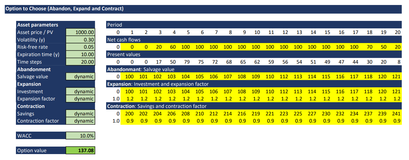
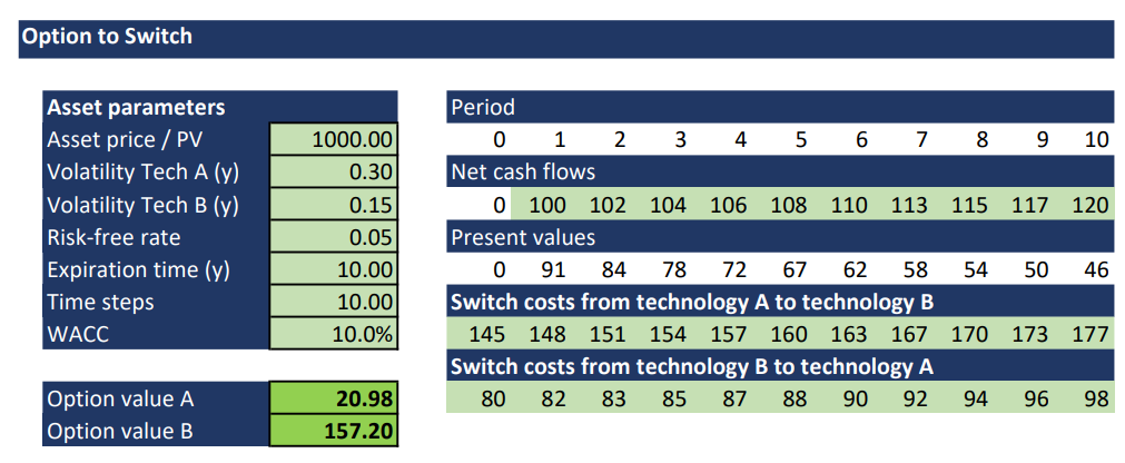
In this post I want to give a simple example of a choose option valuation. The considered project lasts 10 years, the WACC of the contribution (market) cash flows is 10.0% and constant over time. The contribution cash flows are shown in the graph below. Let the risk free rate be 5.0%. The project provides 3 options: 1) Option to expand with an investment of 100 kEUR (increasing with an inflation rate of 2% per year). The contribution cash flows would be increased by 20%, if managements invests in the expansion. 2) Option to abandon the project with a salvage value of 100 kEUR (increasing with an inflation rate of 2% per year) and 3) Option to contract with a savings of 200 kEUR (increasing with an inflation rate of 2% per year) and a contraction factor of 0.9. DCF analysis provides a present value of the market contribution cash flows of 1 million EUR. A Monte-Carlo-Simulation shows a project volatility of 0.30. We analyze this choose option with the binomial approach of Cox-Ross-Rubinstein. As time periods we take two time steps per year, so that you can read the figures in the lattice properly. For higher accuracy we could take smaller time periods anytime.

Choose Option Valuation

We want to give answers to the following questions: What is the value of this option to choose? When do we have to take which option to get the maximum value added for the project?

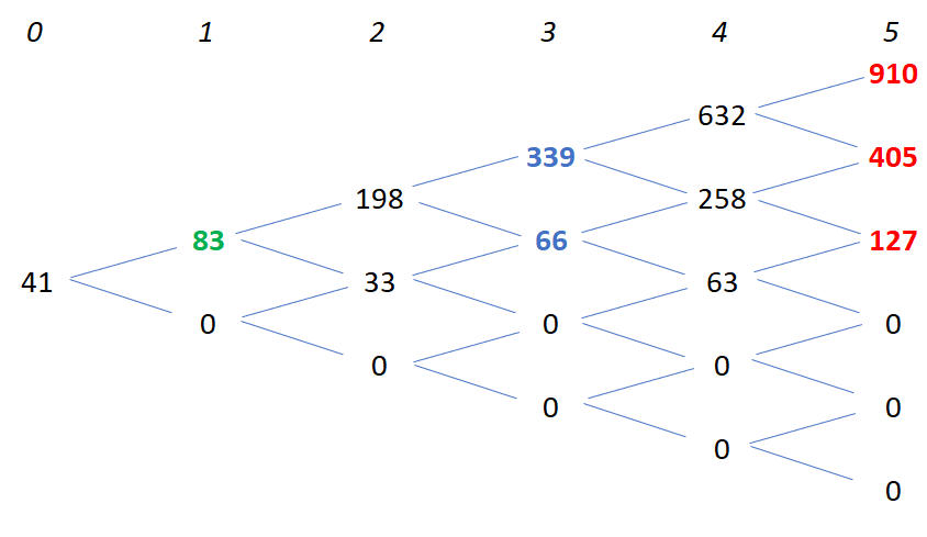
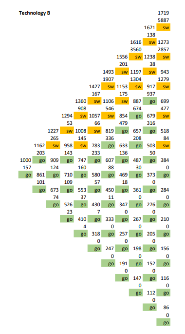
We take the binomial approach from Cox-Ross-Rubinstein to solve that issue. Following you can have look at the binomial lattice. The first value of each node is the value of the underlying (market contribution cash flows). The sevond value is the value of the options at this node. In the third line you can see whether you have to take an option and which option you have to take. “exp” means to invest in the expansion of the project, “go” means to take no option at this node and “con” means to invest in the contraction of the project.

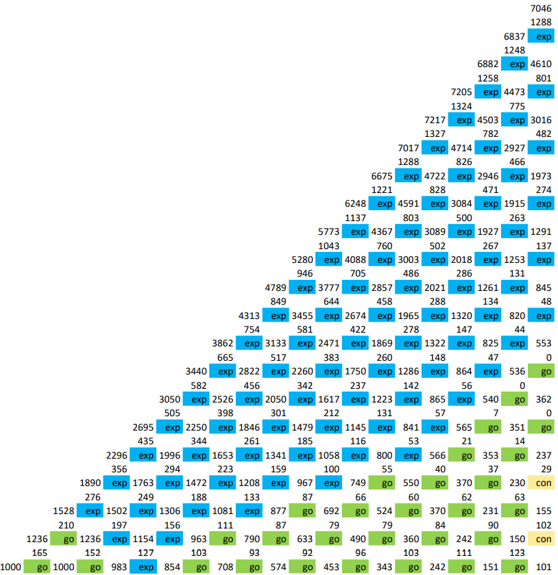
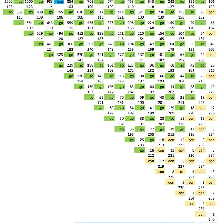
The total value of the three options is 137 kEUR. That is the maximum investment that should be done for the three options in sum. The option to abandon is not taken in any node. That means that you should not invest in this abandonment option. In the first year you should not take any option, let the project evolve. In the second year there might be the first opportunities to take the expansion option. In the following years the expansion option is a good opportunity in case of positive cash flow development. Your project controlling should have a look at the cash flow development and go the right path through the lattice over time. In the first six years the contraction option provides no addition value to the project. But in the last three years of the project the contraction option becomes more important.

Note that this choose option adds a value of 137 kEUR to the project. That means that the NPV of the classical DCF analysis can convert from negative to positive because of the additional value. That could lead to a reconsidering of the project decision. The ENPV (expandedNPV) is the NPV of the project plus the value of the choose option.

Additional Remarks

I constructed the event tree from the project’s contribution cash flow volatility out of a Monte-Carlo-Simulations. Of course you can also create the nodes of the event trees by calculating the time values of the outstanding contribution cash flows explicitly. Discussion with management and marketing can provide the required cash flows and probabilities of the event tree.

This option to choose combines the three options of expansion, contraction and abandonment. This example also shows that the value of various options is not the sum of its individual options. Although the option to abandon has an option value by itself, it contributes no additional value to the option to choose, because it is not required in any node. Analytical valuation methods like Black-Scholes-Merton cannot provide exact solutions for such interdependent options.

Option to Switch Example

Problem Framing

In this post I want to give a simple example of a swich option valuation. The considered project lasts 10 years, the WACC of the contribution (market) cash flows is 10.0% and constant over time. The contribution cash flows are shown in the graph below. Let the risk free rate be 5.0%. The project provides 2 operation modes (possibilities), one with technology A and the other with technology B. A Monte-Carlo-Simulation of technology A shows a project’s contribution cash flow volatility of 0.30. The corresponding Monte-Carlo-Simuation of technology B provides a project’s contribution cash flow volatility of 0.15. We analyze this switch option with a binomial approach. As time periods we choose one time step per year, so that you can read the figures in the lattices. For higher accuracy we could take smaller time periods anytime. The present value of the project market contribution cash flows is 1 million USD. Switch costs from technology A to B start with 145 kUSD, from technology B to A start with 80 KUSD. These costs increase with an inflation rate of 2.0%.

Switch Option Valuation

We want to give answers to the following questions: What is the value of this option to switch between technology A and technology B? How much can we invest in this flexibility keeping a positive added value to the project? And when do I have to switch between the 2 technologies to get the maximum value added?

We take the binomial approach from Cox-Ross-Rubinstein to solve that issue. Following you can have look at the binomial lattices for both technologies. The first value of each node is the value of the underlying (market contribution cash flows), the sevond value is the value of the switch option at the corresponding node. In the third line you can see whether you have to switch to the other technology or not (“sw” means to switch, “go” means to stay in the technology).

Binomial tree of switch option for technology A

*Binomial tree of switch option for technology* B

The value of the switch option starting with technology A is 21 kUSD. Starting with technology B the switch option value is 157 kUSD. If the investment for the switch option flexibility is below these option values, you should do the investment. If you can choose the starting technology, you should start with B. This results in a higher value added, the corresponding investments not taken into account. In the first year you have to make no switch in any case. In the second year it depends on the cash flow development, if you start with technology A. Switch in the bad case to technology B and stay in technology A in case of positive development. Starting with technology B you should stay there and make no switch, independent of the cash flow development. In the third year you should switch to technology A in the best cash flow development. Analyzing the event/option tree through time in this way provides a guideline for what to do in which year, depending on the cash flow development.

Note that this switch option adds a value of 157 kEUR to the project. That means that the NPV of the classical DCF analysis can convert from negative to positive because of this additional value. That could lead to a reconsidering of the project decision. The ENPV (expanded NPV) is the NPV of the project plus the value of the switch option.

Additional Remarks

I constructed the event tree from the project’s contribution cash flow volatilities out of Monte-Carlo-Simulations. Of course you can also create the nodes of the event trees by calculating the time values of the outstanding contribution cash flows explicitly. Discussion with management and marketing can provide the required cash flows and probabilities of the event tree.

This switch option valuation approach can be applied to many problems with different operation possibilities. Switch options are compound options with path-dependency. They are a good examples that real options can be more complicated than financial options. Analytical valuation methods like Black-Scholes-Merton cannot give you a solutions for problems like that.

Replication Portfolio in Binomial Model

In this post I a want to give a short derivation of the replication portfolio and the risk neutral probabilities in the binomial model from Cox-Ross-Rubinstein. Let $V$ be the value of the underlying asset in $t_0$ . In a project or investment this might be the present value of the project’s contribution (market related) cash flows. The positive development of $V$ at time $t_1$ , $V^+$ , occurs with probability $p$ , the negative development with value $V^-$ in $t_1$ with probability $1-p$ . The twin security of the underlying in the open market takes a similar notation $S$ , $S^+$ , $S^-$ , $p$ . We consider an option with option value $E$ in $t_0$ that leads to an option value of $E^+$ in the upper state $V^+$ and to an option value of $E^-$ in the lower state $V^-$ . As result we are searching the option value $E$ at time $t=0$ .

Next we replicate the option value in $t_1$ by a portfolio of $n$ shares of twin security $S$ partly financed by borrowings of amount $B$ at the risk-free rate $r$ . The values of the upper and lower state in $t_1$ are $E^+=nS^+-\left(1+r\right)B$ and $E^-=nS^--\left(1+r\right)B$ .

In efficient markets there exist no profitable arbitarge opportunities. Therefore the outcome of the option value $E$ in $t=1$ must be the same in the upper and in the lower state. Setting $E^+-nS^+=E^--nS^-$ we get:

$n=\frac{E^+-E^-}{S^+-S^-}$

Replacing $n$ in the previous equations we obtain the value borrowed at the risk-free rate r:

$B=\frac{1}{1+r}\frac{{E^+S^--E}^-S^+}{S^+-S^-}$

The law of one price tells us that the value of assets that lead to the same cash flows must be the same. That means that the value of the option at time $t_0$ must be the same as the value of the portfolio at time $t_0$ . Therefore we can set $E=nS-B$ . With that we calculate the value of the option in $t_0$ :

$E=\frac{\left(\frac{S\left(1+r\right)-S^-}{S^+-S^-}\right)E^++\left(1-\frac{S\left(1+r\right)-S^-}{S^+-S^-}\right)E^-}{1+r}$

We create a new variable $p^\prime$ to simplify the previous expression.

$p^\prime=\frac{S\left(1+r\right)-S^-}{S^+-S^-}$

Hence we obtain:

$E=\frac{p\prime E^++\left(1-p\prime\right)E^-}{1+r}$

$p^\prime$ can be interpreted as probability for $E^+$ , $1-p^\prime$ for $E^-$ . $p^\prime$ and $1-p^\prime$ are known as risk-neutral probabilities. Note that the value of the option does not explicitly involve the actual probabilities $p$ and $1-p$ of the underlying. Instead, it is expressed in terms of risk-neutral probabilities. They allow to discount the expected future values at the risk-free rate.

Discounting at the risk-free rate is the main difference between decision tree analysis (DTA) and contingent claim analysis (CCA) or real options analysis (ROA). DTA does not take into account that the risk of the cash flow streams changes when you consider options and opportunities. ROA implements this issue correctly.

WACC, Return Rates & Betas with Debt

Joachim Kuczynski, 02 April 2021

In this post I want to summarize some interesting results concerning equity return rates , betas and WACC of a levered company. Regarding the market value balance sheet of a firm we can state that the value of the unlevered firm VU plus the present value of the tax shield VTS must be the same as the sum of levered equity E and debt D:

$VU+VTS=E+D$

Further the rates of return on each side of the balance sheet are the weighted average of the component rates of return:

$r_A\frac{VU}{VU+VTS}+r_{TS}\frac{VTS}{VU+VTS}=r_E\frac{E}{E+D}+r_D\frac{D}{E+D}$

Substituting VU in the rate of return expression we get a general form of the equity return rate:

$r_E=r_A+\left(r_A-r_D\right)\frac{D}{E}-\left(r_A-r_{TS}\right)\frac{VTS}{E}$

Consequently the general form of CAPM beta is given by:

$\beta_E=\beta_A+\left(\beta_A-\beta_D\right)\frac{D}{E}-\left(\beta_A-\beta_{TS}\right)\frac{VTS}{E}$

The WACC is defined as the weighted average of equity and debt return rates including tax shield at corporate income tax rate $T_C$ . If the tax shield savings are proportional to the taxes paid (see WACC with Tax Shield), the WACC is given by:

$WACC=r_E\frac{E}{E+D}+r_D\left(1-T_C\right)\frac{D}{E+D}$

Substituting the equity return rate we get a general form of the WACC:

$WACC=r_A\left(1-\frac{VTS}{V}\right)-r_DT_C\frac{D}{V}+r_{TS}\frac{VTS}{V}$

$r_A$ , $r_D$ , $r_{TS}$ are the return rates of the unlevered asset, debt and tax shield. V and VTS are the values of the levered firm and the tax shield. D is the amount of debt, V is the value of the levered firm, namely the sum of equity and debt.

Modigliani and Miller: Constant debt value
If the firm keeps its dept value D constant, there are no specific market risks concerning the tax shield. Therefore we can set the tax shield discount rate $r_{TS}$ equal to the debt discount rate, $r_D$ . The tax shield present value with constant debt D is:

$VTS=\sum_{j=1}^{\infty}{DT_C\left(\frac{1}{1+r_D}\right)}^j=\frac{DT_C}{r_D}$

Hence we get simplified expressions for equity return, equity beta and WACC:

$r_E=r_A+\left(r_A-r_D\right)\frac{D}{E}\left(1-T_C\right)$

$\beta_E=\beta_A+\left(\beta_A-\beta_D\right)\frac{D}{E}\left(1-T_C\right)$

$WACC=r_A\left(1-T_C\frac{D}{E+D}\right)$

Assuming that debt interest rate does not depend on the market return rate (CAPM) we can set $\beta_D=0$ . Hence we get the well-known Hamada equation for levered beta:

$\beta_E=\beta_A\left(1+\frac{D}{E}\left(1-T_C\right)\right)$

It is important to realize that Hamada’s equation is only valid if the value of debt is kept constant over time.

Harris and Pringle: Constant leverage ratio
Constant leverage ratio means that debt value is proportional to the value of the unlevered firm. According to Harris and Pringle that results in $r_{TS}=r_A$ .

$r_E=r_A+\left(r_A-r_D\right)\frac{D}{E}$

$\beta_E=\beta_A+\left(\beta_A-\beta_D\right)\frac{D}{E}$

$WACC=r_A-r_DT_C\frac{D}{E+D}$

But we have to take care. Miles and Ezzell, Arzac and Glosten have shown that you have a tax shield discount rate of $r_D$ in the first period, and of $r_A$ in the following periods to have a constant leverage ratio over time. The premise of $r_{TS}=r_A$ does not hold.

Miles and Ezzell
With a perpetuity growing rate g of debt and discounting in the first period with $r_D$ instead of $r_A$ we obtain:

${VTS}^{ME}=\frac{Dr_DT_C\left(1+r_A\right)}{\left(r_A-g\right)\left(1+r_D\right)}$

Harris and Pringle
Taking the formula of Miles and Ezzell and setting $r_TS$ equal to $r_A$ in the first period, we get the a simplified expression for $VTS$ :

${VTS}^{HP}=\frac{Dr_DT_C}{\left(r_A-g\right)}$

General debt ratio
If the amount of leverage is flexible and not constant or growing with a constant growth rate over time, the previous formulas do not work. In this case you have to use the APV method, in which you calculate the tax shield in each time period seperately.

Baldwin Rate of Return | MIRR

Joachim Kuczynski, 05 March 2021

Baldwin rate definition

The modified internal rate of return (MIRR), or Baldwin rate of return respectively, is an advancement of the internal rate of return (IRR). But also the MIRR can be misleading and can generate false investment decisions. The MIRR is defined as:

$MIRR=\sqrt[n]{\frac{\text{FV(contribution cash flows,WACC)}}{\text{PV(invest cash flows, financing rate)}}}-1$

FV means the final value at the last considered period, PV stands for the present value.

Pitfalls of the Badwin rate

These points have to be considered carefully when applying the MIRR:

Cash flows in different countries, with different currencies, equity betas, tax rates, capital structure, etc. should be evaluated with specific risk-adjusted discount rates. In MIRR the project is profitable, if the rate of return is higher than the required WACC. But which WACC do we mean in projects with various differing cash flows ? No diversification of cash flows can be taken into account in MIRR. But that is crucial in evaluating international projects.
You need premises about the reinvestment rate of the contribution cash flows that affect the profitability of the project. These premises are not required in the (e)NPV concept. Hence you add an additional element of uncertainty in your calculation when using the MIRR, without any need.
Reinvesting contribution cash flows (numerator of the root) with the risk adjusted WACC means that the return of the project increases when the project risks and WACC increases. That cannot be true. In pinciple you should not use key figures that require assumptions about reinvestment return rates. You are evaluating a certain project and not of other unknown investment sources. In general you can discount all cash flows with its appropriate discount rate and capitalize it to the last period.
Does capitalizing (or rediscounting) a cash flow with a risk-adjusted discount rate to a future period make sense in general? I do not think so. To rediscount cash flows with a risk adjusted discount rate including a risk premium means that you are increasing the risk of the project. The project does not remain the same, because its risk increases. Only taking a riskless discount rate for reinvestments would not increase the risk of the project. The MIRR comes from a classical perspective with no risk adjustment of the discount rates. If you are using risk-adjusted discount rates, you are mixing two concepts that do not fit.
An additional positive cash flow must improve the profitability of the project. If you add an additional, small cash flow in an additional period $n+1$ , the Baldwin rate can decrease. This is because the number of periods increases and the value of the root decreases. Cases that lead to wrong results are not acceptable for decision key figure.
If you have e.g. an after sales market with small positive cash flows, the Baldwin rate decreases by considering these cash flows in your calculation. This is because the number of periods increases and the $n$ -th root decreases. Thus an after sales market cannot be implemented in your calculation.
You have to define clearly, which cash flow is in the numerator and which is in the denominator of the root. There is no clear and logic distinction. Thus you can find different definitions in literature. Anyway avoid to take balance sheet definitions of “investment”. Note that besides investments also fixed costs and leasing payments have to be discounted with a default free discount rate in general.
You cannot compare mutual exclusive investment projects, if the investments or the project periods are different.
You can also not evaluate investment projects with negative value contribution to the firm. But anyway such projects exist and have to be decided.
All cash flows should be considered as expected value of a probability distributions. The expected value of the Baldwin rate is not the Baldwin rate of the expected values of the cash flows.

Conclusion

The (e)NPV concept is much better than the MIRR or Baldwin Rate of Return. The (e)NPV does not have all the pitfalls mentioned above. Further you can also evaluate and compare value-loosing investment alternatives and do not need any premises about reinvestment rates. There are only disadvantage of the MIRR / Baldwin rate compared to the (e)NPV, try to avoid the application of MIRR / Baldwin rate.